A $28 Trillion Mistake

Major errors in two papers at the center of the climate liability movement

Roger Pielke Jr., 06.11.2026

The findings in brief

A 2022 paper (Callahan and Mankin 2022, CM22) in Science Advances linked hot spells to economic growth in more than 1,200 regions and estimated $5 trillion to $29 trillion in global losses from “human-caused increases in heat waves.” A follow-up 2025 paper (Callahan and Mankin 2025, CM25) in Nature allocated the emissions of 111 fossil fuel companies under that methodology to argue that those companies were responsible for $28 trillion in economic losses, and to allocate those losses to individual companies.

Motivated by and building on a reanalysis of Callahan and Mankin 2022 by statisticians Abraham Wyner and Ryan Brill, I reproduced CM22 and CM25 with the authors’ data and code, and have found major errors in each.

This post reports what I found and shares my methods, data, and code, so others can check my work — downloads are available at the bottom. I argue that there is a very strong case for the retraction of both CM22 and CM25.

CM25 characterize their analysis as supporting climate litigation:

Will it ever be possible to sue anyone for damaging the climate? Twenty years after this question was first posed, we argue that the scientific case for climate liability is closed. Here we detail the scientific and legal implications of an ‘end-to-end’ attribution that links fossil fuel producers to specific damages from warming.

I have often argued that an index of global temperature is not a cause of weather or impacts — which is the core of the CM methodology. However, in the detailed analysis reported in this post, I replicate their work on its own terms, and find that both papers are fatally flawed — even taking them at face value.

Specifically, I found four errors in Callahan and Mankin’s 2025 paper that when corrected eliminate their headline conclusion:

• Temperature scale. Callahan and Mankin get results that differ widely depending on whether temperatures are expressed in Celsius, Fahrenheit, or Kelvin. They multiply each hot-spell temperature by the region’s average temperature with results dependent on where zero falls in each measure. When I repeat their calculation using each temperature scale, I get losses of $28 trillion in Celsius (as they did), $43 trillion in Fahrenheit, and $359 trillion in Kelvin.
• Currency. Callahan and Mankin measure growth in US dollars, so they mistake a national currency crash for a collapse in national production. When growth in local currency after inflation is used under their method, their headline result is cut in half.
• Data breaks. In 2001, the regional data for Honduras switched to a new source. In Callahan and Mankin’s data, output in 14 Honduran regions jumps 76% to 395% that year, even though the national economy did not grow. Callahan and Mankin treat that statistical artifact as real economic growth. Removing those 14 data points, out of more than 20,000, cuts their $28 trillion result by a third.
• Lag alignment. Callahan and Mankin line up the delayed effects of hot spells after skipping years with missing data, so some “one-year” delays span several calendar years. Properly aligning years raises their headline result to $39 trillion.

A reproduction of their methodology with all four errors corrected results in totals from a $5 trillion gain to a $2 trillion loss, scattered around zero and nowhere near the published $28 trillion loss.

By the standard Nature applied in the December 2025 Kotz et al. retraction, the journals have ample justification to retract both papers. The editors of Nature and Science Advances now face a test of their publication standards.

I invite Callahan and Mankin to respond to this analysis and I will be happy to publish their response here at The Honest Broker.

The analysis in detail

Callahan and Mankin claim to attribute specific losses to specific companies. With their data and code, I find no support for that claim. With correction of clear errors in the application of their methods or the use of equally reasonable choices in applying their method, I can turn their reported $28 trillion loss into net gains, or increase the 2025 total and the 2022 loss.

I found four errors in Callahan and Mankin’s 2025 calculation, and correct each to assess the significance for their reported results:

• Temperature scale. Callahan and Mankin compute damages that vary with the zero point of the temperature scale.
• Currency. Callahan and Mankin measure growth in US dollars at market exchange rates, so they count currency crashes as lost production.
• Data breaks. Callahan and Mankin keep 24 country-years with a change of data source, including Honduras in 2001.
• Lag alignment. Callahan and Mankin line up delayed effects after skipping years with missing data, so some “one-year” delays span several calendar years (detailed in the Appendix).

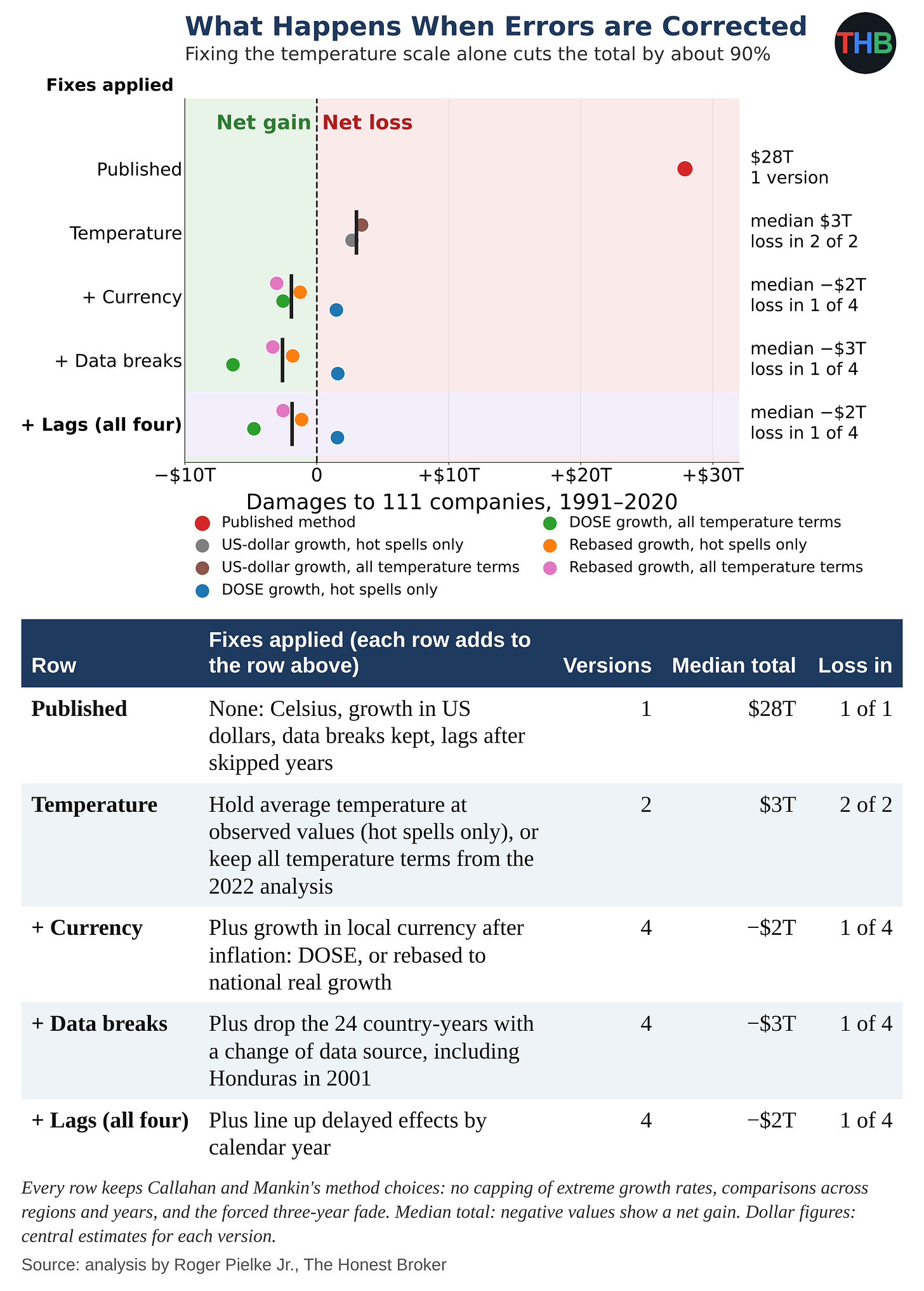
The figure below summarizes what happens when these errors are corrected — the $28 trillion loss disappears.

In each row in the figure, I add one fix to the row above and otherwise implement the CM25 methodology. I mark each version of the 2025 total with a dot and the median of each row with a black bar. The temperature fix alone cuts the total by about 90%, to $3 trillion. With the currency fix added, the median result turns into a $2 trillion gain. With all four fixes, results range from a $5 trillion gain to a $2 trillion loss.

Some technical details: I concluded that there is more than one reasonable fix for two of the errors, so I tested each one. For the temperature scale, I used two fixes. In the first, I held each region’s average temperature at its observed values and let only hot spells change, an option Callahan and Mankin had in their 2025 replication package. That fix counts only the effect of hotter hot spells, the quantity at the center of their claim. In the second, I kept every temperature term from their 2022 statistical analysis. Besides multiplying hot spells by average temperature, Callahan and Mankin estimated separate terms for average temperature by itself. When I move the zero point of the scale, the separate terms shift by an amount that offsets the change in the product, so the choice of temperature scale no longer affects the result. With either fix, I get the same answer in Celsius, Fahrenheit, and Kelvin. For currency, I also used two fixes. In the first, I replaced Callahan and Mankin’s growth figures with DOSE, a database of regional output in local currency after inflation from the Potsdam Institute for Climate Impact Research and the Mercator Research Institute. In the second, I kept Callahan and Mankin’s regional figures but adjusted them to match, on average, each country’s real growth rate after inflation, taken from the Penn World Table figures in their 2022 dataset; with that fix, I keep their regional detail and remove the currency swings. I paired each temperature fix with each currency fix — thus, four versions in all. The results are robust to these choices.

Beyond the obvious errors, Callahan and Mankin also made three methodological choices that could reasonably make differently:

• Comparisons across countries. Callahan and Mankin compare regions from different countries with one another. That creates a problem. When Indonesia’s currency crashed in 1997, every Indonesian province looked poorer on paper at the same moment. If Indonesia also had a hot summer that year, a comparison with other countries would blame the heat for losses that the currency crash caused. So I implemented a fairer comparison: I compared each region only with its neighbors in the same country in the same year. Indonesian provinces in 1997 all lived through the same currency crash, the same government and the same national economy. When I made the comparison that way, I found no heat effect.
• Extreme growth rates. Callahan and Mankin keep every growth rate in their data, including jumps and drops of more than 100% in a single year, many of them data artifacts like the Honduran break. A handful of such extremes can sway the results. As an alternative, I capped the most extreme 1% of growth rates at each end to limit the influence of outliers.
• A forced fade. Callahan and Mankin estimate the effect of a hot spell on growth in that year and the five years after, then impose a pattern in which the harm builds for three years and — seemingly arbitrarily — vanishes by the third year after the hot spell. As an alternative, I used Callahan and Mankin’s own estimates of a hot spell’s effect on growth in each of the six years, without forcing that effect to vanish by the third year..

In the figure below, I started from the calculation corrected for the four errors detailed above and applied the three alternative methods choices, alone and in combination. In each row, I apply a different set of alternatives to the corrected calculation and again show four versions, one for each pair of temperature and currency fixes.

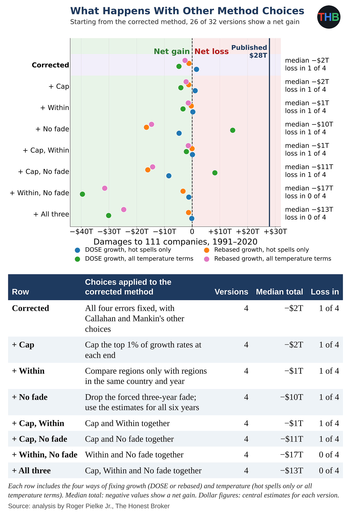
Across the 32 versions showing the results based on different methodological choices, I got a net gain in 26. I found the largest effect in the fade choice: when I drop the forced fade, the median moves from a $2 trillion gain to a $10 trillion gain. With all three alternatives, I found a net gain in all four versions. Among the 32 versions, I found no loss larger than $15 trillion.

If Callahan and Mankin had measured a real effect of extreme heat, we would expect the corrected versions to agree on a loss of some size. I found them scattered around zero, mostly on the side of a net gain, which — taken at face value — would assign economic benefits to the emissions of the 111 companies, which might seem like nonsense.

A yardstick: the Kotz retraction

In December 2025, Nature retracted Kotz et al. which projected a 19% loss in world income by 2050 from climate change.

In replication, others identified bad data from one country, Uzbekistan, and found that Kotz et al. had ignored the shared shocks of neighboring regions in their uncertainty ranges. After fixing both, along with other problems, the authors widened their likely range for the 2050 loss from 11–29% to 6–31%. The authors judged those changes “too substantial for a correction,” and Nature withdrew the paper.

I found similar problems in Callahan and Mankin’s 2025 paper, in comparable or larger form, along with three other problems.

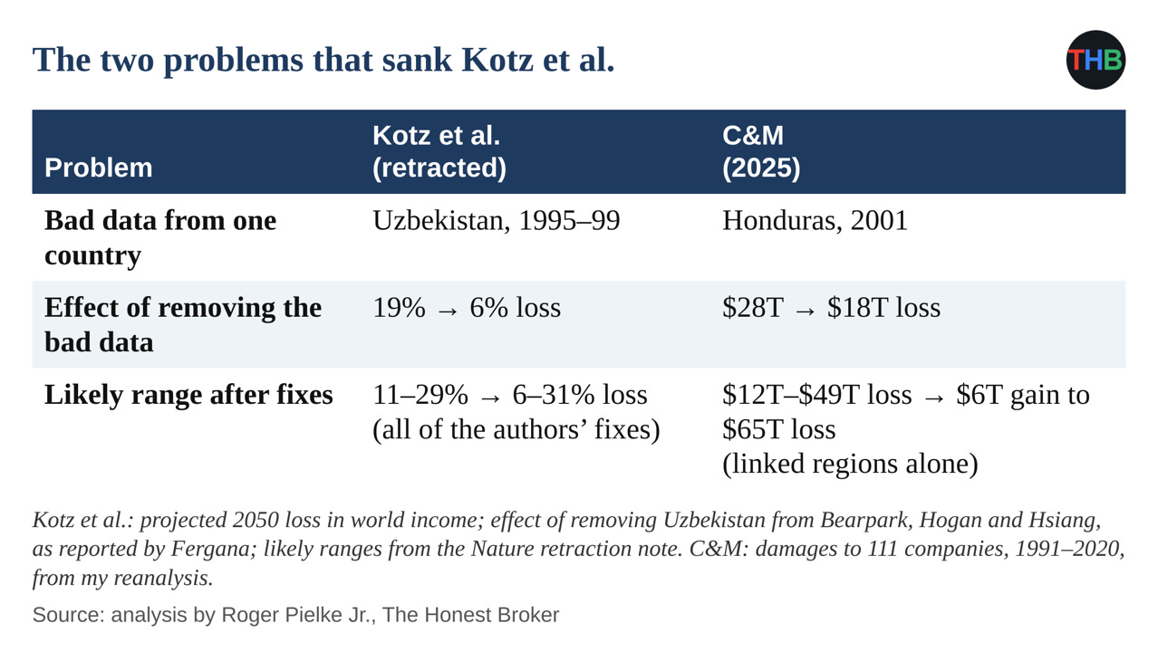
By the standard Nature applied to Kotz and colleagues, the journals should retract both Callahan and Mankin papers.

Why no fix can rescue the method

Up to this point, I have taken Callahan and Mankin’s methods at face value. However, I also reject their starting assumption that a metric of global average temperature causes weather or economic impacts.

No researcher can rescue this approach with better data, more clever statistics, or a different methodology.

As I argued earlier this year:

If the problem were merely technical — better data, longer panels, more clever econometrics — the field could reasonably expect to close in on the truth over time. If the problem is conceptual — that the top-down approach is correlating two downstream summaries with no causal structure between them — then more data and cleverer methods will not help. The field will continue producing numbers and those numbers will generate headlines, but those numbers, whatever they mean, don’t tell us anything meaningful about how future changes in weather might affect future economic activity.

Below, I describe in a lot of detail the two papers and my tests, and then each problem, with figures and tables. At the bottom please find a detailed methods document, a spreadsheet, and Python code that can be used to replicate my replication.

This analysis was a big one — Before you go, please click the “❤️ Like” button!

Comments, questions, critique all welcomed!

Leave a comment

Methods Appendix

How I did the work. I used Claude for the coding. To ensure quality, I ran five separate analyses, each with independently written code and instructions to refute the findings, and got the same core results; in two further audits (think of this as a “peer” review), I checked every claim against the papers, the data, and the code.

With a separately written program, I reproduced each 2022 dollar figure within 4%, except the version with average temperature held at observed values, which I checked against the authors’ stored result ($1.91 trillion against my $1.94 trillion). For each bar in the 2025 forks figure and each row in the tables, I ran 10,000 simulations of the full 2025 calculation; for each bar in the 2022 figure, 1,000 simulations of the 2022 calculation.

This Methods Appendix and the Method Document were drafted by Claude under my direction and heavily edited by me to ensure accuracy and consistency.

Overview of CM22 and CM25. In 2022, Christopher Callahan and Justin Mankin of Dartmouth College published a paper in Science Advances in which they compared each year’s economic growth in regions around the world with the temperature of each region’s hottest five days. Callahan and Mankin estimated that link from more than 1,200 regions in 68 countries. They reported lower growth in warm regions after hotter hot spells, and with that statistical link they estimated losses to the world economy of $5 trillion to $29.3 trillion from human-caused increases in extreme heat between 1992 and 2013, with the largest losses in the poorest regions.

In April 2025, Callahan and Mankin applied that statistical link in a paper in Nature that assigned $28 trillion in economic losses from extreme heat between 1991 and 2020 to the emissions of 111 fossil fuel companies. They put Chevron’s share at $791 billion to $3.6 trillion, with similar amounts for Saudi Aramco, Gazprom and ExxonMobil, and declared that “the scientific case for climate liability is closed.”

The chain of causality that they assert is shown in the figure below.

Callahan and Mankin built the two papers as one chain of calculation. In 2022 they estimated the link between heat and growth; in 2025 they fed company emissions through that same link to produce dollar figures. So any problem in the 2022 link affects every company figure in the 2025 paper. Callahan and Mankin also used the same structure for the dollar calculation in both papers, so I found the same dollar-calculation problems in both papers.

Callahan and Mankin built their 2025 total of $28 trillion in loss in five steps:

1. Emissions. They took each company’s historical emissions from the Carbon Majors database.
2. Warming. They used FaIR, a simplified model that converts emissions into estimates of global warming, to estimate each company’s share of the warming.
3. Regional heat. They used patterns from climate models to translate global warming into changes in each region’s hottest five days of the year.
4. Heat and growth. They applied the statistical link from their 2022 paper to turn changes in hot spells into changes in each region’s growth.
5. Dollars. They converted the lost growth into dollars using each region’s income.

For each company, Callahan and Mankin compared the world as it happened with an imagined world without that company’s emissions and attributed up the difference in income to that company’s emissions.

In September 2026 statisticians Abraham Wyner and Ryan Brill of the University of Pennsylvania published a reanalysis of the CM22 statistical link. Economists expect neighboring regions to share good and bad years, and nearby years to follow similar patterns.

Once Wyner and Brill allowed for those connections, they found far less precision in Callahan and Mankin’s estimates. When Wyner and Brill dropped a few influential countries or years, they could erase the heat effect or reverse its direction. When they grouped regions within countries, they found an effect 67% to 90% smaller, with uncertainty ranges that included zero, and they predicted growth no better with the extreme-heat measure than without that measure.

Wyner and Brill examined only the 2022 statistical link. Their analysis motivated me to perform a much more comprehensive replication of CM22 and CM25 reported in this post.

How I replicated the two papers. I reproduced both papers with the authors’ data and code. I matched the $28 trillion and every company figure in the 2025 paper, and the $16 trillion average loss in the 2022 paper.

Then I tested the papers at two levels:

• The 2022 link. I refit Callahan and Mankin’s 2022 statistical analysis with each correction and choice and measured the change in their main result, the three-year effect of a hotter hot spell on growth in a region with an average temperature of 25°C.
• The dollar calculations. I ran each version of the link through the dollar calculations in both papers: the 2022 global loss of $16 trillion and the 2025 company total of $28 trillion.

In the main body of this post I focus on CM25 because Callahan and Mankin used it to assign losses to individual companies. Under each problem discussed below, I report the effect on the 2025 total and on the 2022 paper, and in a chart near the end I show the consequences of each change for the 2022 loss estimate.

I found problems at different points in the two papers:

• Currency crashes, data errors and linked regions: Callahan and Mankin built these problems into the 2022 statistical link, so I found their effects in both papers.
• The temperature scale: Callahan and Mankin made this error in the dollar calculations of both papers. When I refit the 2022 statistical analysis on each scale, I get the same fit.
• The posted code: when I ran the code Callahan and Mankin posted with each paper, I could not reproduce the published result.

In April I argued that researchers who conduct statistical studies of this kind measure no real, causal quantity.

Here I set that view aside and take Callahan and Mankin on their terms, with a narrower set of questions: Are there any obvious errors in their methods? And, if the method worked as they say, how much would their numbers change under small, reasonable revisions?

My alternative figures should not be interpreted as a better estimate of the costs of extreme heat. I am simply testing the stability of the published results when errors are corrected and other plausible methodological choices are made.

I fully reject the notion that an index of global temperature causes either weather or weather impacts, and any methodology built on such causality is conceptually flawed.

The next sections go into more detail on each of the problems discussed in the main body of this post.

Problem 1: An answer that depends on the temperature scale

Scientists describe the same temperature using Celsius, Fahrenheit and Kelvin scales with different zero points: water freezes at 0°C, 32°F and 273.15 K. With Callahan and Mankin’s calculation, I get a different dollar figure for the same temperature under each scale, because their methodology is dependent upon where zero lies in each scale.

Callahan and Mankin assume that a hot spell does more harm in a place that already is hot, so a heat wave in Lagos hurts more than one in Oslo. To build that assumption into their calculation, they multiply two numbers together: the temperature of a region’s hottest five days and the region’s average temperature.

Why multiplying temperatures causes trouble. The answer to a multiplication depends on where the thermometer puts zero. Celsius puts zero at the freezing point of water; Kelvin puts zero at absolute zero, 273 degrees lower. A one-degree warming has the same size on both scales, but the number it gets multiplied by does not.

The setup. Take one region. Its hottest five days average 30°C, and its average temperature is 20°C. Callahan and Mankin estimate damages by comparing the world as it happened with an imagined world without a company’s emissions. Suppose that in the imagined world, the region’s average temperature would be one degree cooler: 19°C.

In Celsius. Callahan and Mankin multiply the hot-spell temperature by the average temperature.

• Actual world: 30 × 20 = 600
• Imagined world: 30 × 19 = 570
• Difference: 30

In Kelvin. The same weather in Kelvin is 303 K for the hot spell, 293 K for the actual average and 292 K for the imagined one.

• Actual world: 303 × 293 = 88,779
• Imagined world: 303 × 292 = 88,476
• Difference: 303

The result. The weather stays identical, and the one-degree difference between the two worlds stays identical. Yet the difference that drives the damage figure grows tenfold, from 30 to 303, only because Kelvin puts zero 273 degrees lower than Celsius.

How the difference becomes dollars. Callahan and Mankin’s 2022 statistical analysis gives them a number that converts the multiplied term into lost growth. Call it the conversion factor. For each region and year, the damage calculation takes the difference between the two worlds and multiplies it by that factor to get the growth the region lost. The conversion factor comes out the same on both scales, because a one-degree change has the same size in Celsius and Kelvin, so the factor does nothing to correct for the zero point. Suppose for illustration that the factor equals 0.001 percentage points of growth per unit:

• In Celsius: 30 × 0.001 = 0.03 percentage points of lost growth
• In Kelvin: 303 × 0.001 = 0.3 percentage points of lost growth

The same weather now produces ten times the lost growth in Kelvin. Callahan and Mankin then add up each region’s lost growth year after year, convert the shortfall in income into dollars, and sum across regions and companies. Each step carries forward the 10x difference created by the zero point, and that is why the CM25 totals end up at $28 trillion in Celsius and $359 trillion in Kelvin.

Why their 2022 analysis avoided the problem. In their 2022 statistical analysis, Callahan and Mankin did more than multiply the hot-spell temperature by the average temperature. They also included the average temperature on its own, as a separate ingredient with its own conversion factor. That separate ingredient acts as a counterweight.

Return to the example. Switching from Celsius to Kelvin raises the multiplied term’s difference from 30 to 303, an extra 273. When Callahan and Mankin fit their 2022 statistical analysis in Kelvin, the conversion factor on the separate average-temperature ingredient adjusts to subtract exactly that extra 273. The one-degree warming then counts as 303 − 273 = 30 in Kelvin, the same as in Celsius. The statistical analysis fits the data identically on every scale, because the two ingredients always offset each other’s shifts.

Where the 2025 calculation went wrong. In the 2025 damage calculation, Callahan and Mankin kept the multiplied term but dropped the separate average-temperature ingredient. Without the counterweight, nothing subtracts the extra 273, and the choice of scale flows straight into the damages: 30 in Celsius, 303 in Kelvin, and in the end $28 trillion against $359 trillion.

In the table below I also show two other versions:

Hot spells only. In this version, I hold each region’s average temperature at its observed values in both worlds, the actual one and the imagined one without a company’s emissions. The two worlds then differ only in the temperature of their hottest five days. With the average temperature fixed, Callahan and Mankin’s own statistical results already cancel the effect of the zero point, so I get the same answer in Celsius, Fahrenheit and Kelvin: $2.5 trillion. This version measures what Callahan and Mankin say they study, the economic harm from hotter hot spells. They wrote it into their own code as an option, constant_tmean = True, and presented a map of its results (Extended Data Fig. 1) but chose not to report its much smaller loss total.

All temperature terms kept. In this version, I let average temperature differ between the two worlds, as Callahan and Mankin do, but I restore the separate terms for average temperature from their 2022 statistical analysis, the terms they dropped from the 2025 damage calculation. Those terms account for the shift in the zero point, so I again get the same answer on every scale: $3.6 trillion. This version measures the harm from warming as Callahan and Mankin’s full 2022 statistical model describes it, through changes in both hot spells and average temperature.

Both versions fix the temperature-scale error, and they result in much smaller losses, at $2.5 trillion and $3.6 trillion, versus the published $28 trillion. Because both are reasonable fixes, I report them both.

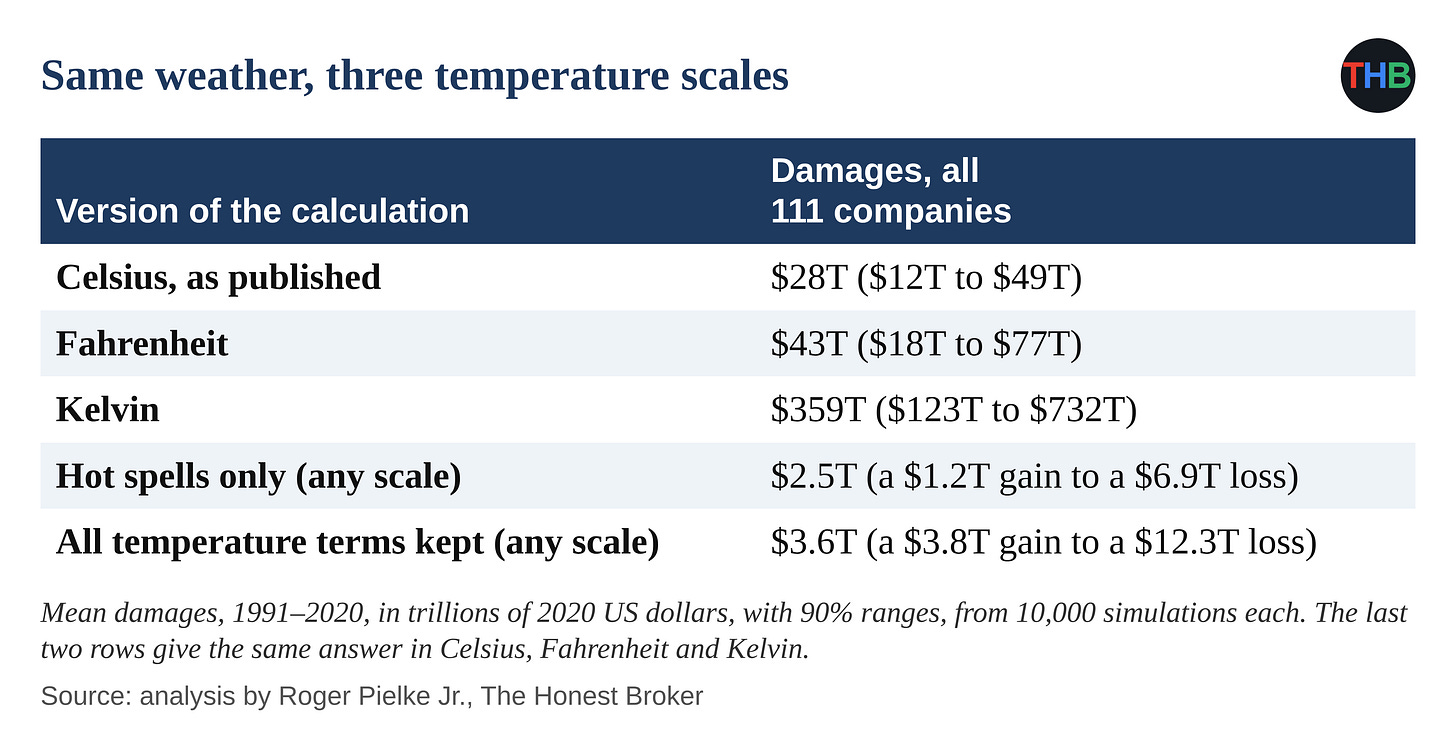
I rank this problem first because it is so obvious, easy to understand, and clearly results in the almost complete elimination of the top line finding of CM25. When a method’s results change 13x with a change of units, the method is clearly flawed.

The temperature-scale error affects dollar figures, not their statistical model. When they turn that model into dollars, in both papers, they drop the separate average-temperature term, and the choice of scale flows straight into the losses: $16 trillion in Celsius and $159 trillion in Kelvin in 2022, and $28 trillion and $359 trillion in 2025. With average temperature held at its observed values, I get $1.9 trillion, 88% less, a version Callahan and Mankin computed and mapped in their supplement (fig. S10) without reporting its dollar total.

Problem 2: Currency crashes counted as economic collapses

Economists measure growth as the change in an economy’s production of goods and services, in local currency after an adjustment for inflation. Callahan and Mankin used a different measure. Kalkuhl and Wenz (2020) converted each region’s output into US dollars at market exchange rates, and Callahan and Mankin, who took those data by way of Kotz and colleagues, adjusted the dollars for US inflation alone in their data-preparation code. In their “growth” figures, Callahan and Mankin therefore mix three things: real changes in production, inflation in the local currency and swings in the exchange rate.

Traders set exchange rates in currency markets, reacting to interest rates, money flowing out of a country, speculation and government decisions. In a currency crash, investors might sell a country’s currency in large amounts and drive its value against the dollar down by a third, a half or more within months, while farmers and factory workers keep producing roughly the same goods. For instance, Indonesian farmers harvest the same rice, but they receive half as many dollars for each sack.

Callahan and Mankin interpret a drop in dollar value as a drop in production. By the end of 1997, traders had cut the value of the Indonesian rupiah against the dollar by about half, and I matched Callahan and Mankin’s Indonesian figures to that end-of-year exchange rate. According to the Penn World Table, Indonesians increased output per person, in rupiah after inflation, by about 3% that year. Callahan and Mankin record a 44% decline for the typical Indonesian province.

The table below shows other examples of how Callahan and Mankin mistakenly interpreted currency crashes as economic collapses.

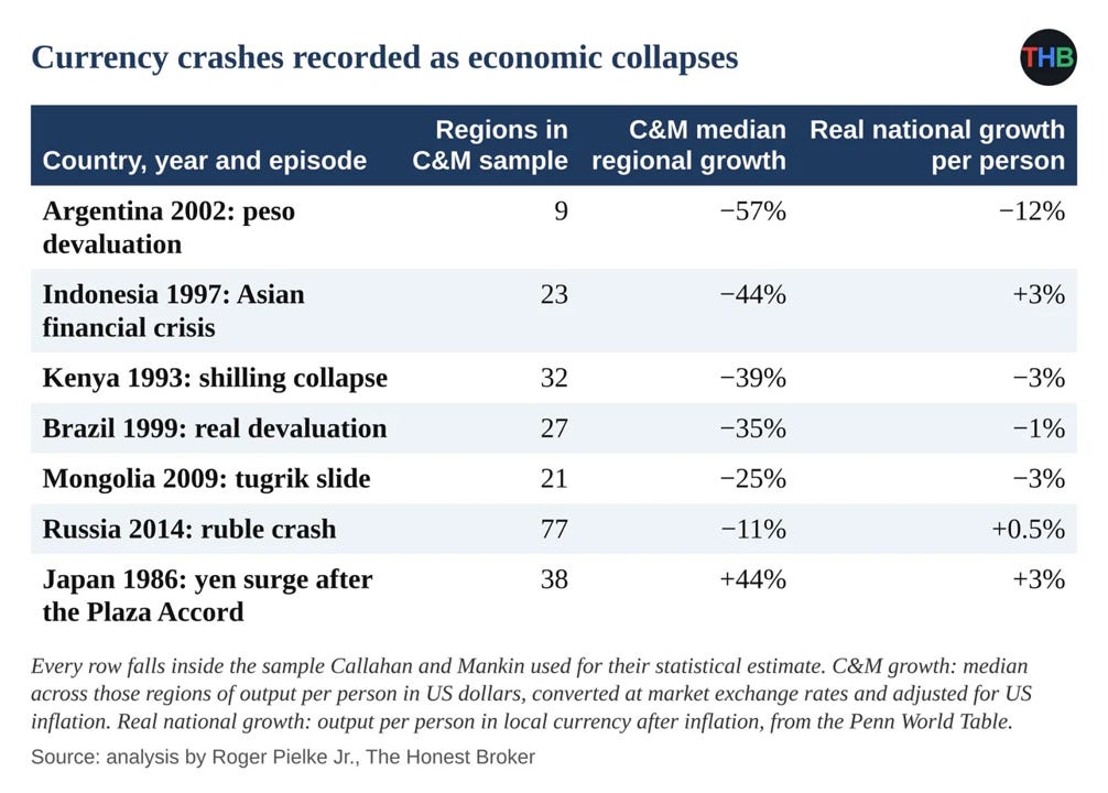
Callahan and Mankin made a category error. They treated a change in the price of a currency as a change in a region’s production of goods and services.

To address this error, I split Callahan and Mankin’s growth figures into real growth in local currency and a remainder of currency swings and inflation, and I reproduced most of their heat effect from that remainder: 73% to 91%, depending on how I split the two. With measures of growth that leave out exchange rates, I found an effect in hot regions 32% to 73% below Callahan and Mankin’s estimate. When I used DOSE, a database of regional output after inflation from the Potsdam Institute and the Mercator Research Institute, in the 2025 calculation, I got $14 trillion in place of $28 trillion.

Problem 3: Data errors like those behind the Kotz retraction

I found errors in Callahan and Mankin’s data like the Uzbek errors behind the Kotz retraction:

• For 2001, Callahan and Mankin record a jump of 76% to 395% in output in every region of Honduras, with no return to earlier levels, in a year of zero growth for the Honduran economy. The compilers of DOSE record a change of data source for every Honduran region that year — meaning that this is a data discontinuity, not an actual jump in growth rates.
• For some Kenyan regions, Callahan and Mankin record income as low as $10 to $50 per person per year, two of them at an identical $10.34 in 1997, along with one-year jumps of 600% to 900%.
• Callahan and Mankin record Uzbek dollar figures that rise with Uzbek inflation. Wenz identified currency-conversion errors as a key reason for the Uzbek problem in the Kotz data — which tipped me off to look at that here.

When I removed the 14 Honduran data points for 2001, out of more than 20,000, I got $18 trillion in place of $28 trillion. When I removed the 24 country-years in which the DOSE compilers record a change of data source, I got $16 trillion. For comparison, Bearpark, Hogan and Hsiang removed Uzbekistan and cut the Kotz projection of the 2050 loss from 19% to 6%.

Problem 4: Uncertainty ranges that include zero

Callahan and Mankin estimated their uncertainty by repeating their analysis thousands of times on random samples of regions, and so treated each of more than 1,200 regions as an independent piece of evidence. People in regions of a country share recessions, currency crashes and policy changes; Indonesians in every province suffered through the 1997 rupiah collapse. By treating such regions as independent, Callahan and Mankin overstated the certainty of their result, the objection Wyner and Brill raised against the 2022 paper.

I repeated the 2025 calculation (without fixing their errors) with four standard statistical methods in which regions of the same country share shocks:

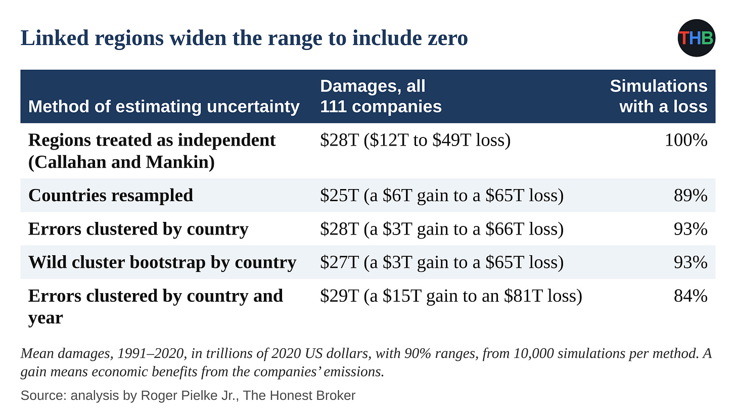
In Callahan and Mankin’s published calculation, I found a loss in all 10,000 simulations. With the four methods that allow for shared shocks, I found a loss in 84% to 93% of simulations, and I got 90% ranges that include zero for the companies as a group and for each of the five largest companies. For the 2022 statistical link, Callahan and Mankin also sampled whole countries, posted those results and showed them in their supplement (fig. S7), along with errors clustered by country (Table S1). They based both dollar calculations, in 2022 and 2025, only on samples of regions.

Two tests from Wyner and Brill

A model with countries and years. In their model, Wyner and Brill grouped regions within countries and linked each year’s shared shock to the previous year’s shock. I rebuilt the model from their paper, fit it to Callahan and Mankin’s data and pushed 1,000 sets of results through the 2025 damage calculation. I get $3.6 trillion, with a 90% range from $0.1 trillion to $8.0 trillion, and I cut Chevron’s figure by 88%. I get a total near the two scale-free versions from Problem 1, about $3 trillion.

Scrambled weather. Wyner and Brill also tested Callahan and Mankin’s heat effect against chance. For each country, they shuffled the order of the weather years and applied the same shuffle to every region in that country. With each shuffle, I kept each country’s weather and economic history and broke any link between a given year’s heat and that year’s growth. I applied their shuffle 400 times and pushed each result through the full 2025 calculation.

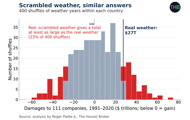
In 23% of the 400 shuffles, I got a total at least as large as the $27 trillion from the real weather, as a loss or as a gain. With scrambled weather, I got totals from a $59 trillion gain to a $70 trillion loss, a range that includes the published total. With Callahan and Mankin’s method, I routinely got totals in the trillions of dollars from weather with no connection to the economic years in question.

Problem 5: Posted code at odds with the published results

When I ran the damage script from the 2025 replication package, I hit a formatting error before the script computed any damages. In the posted script, Callahan and Mankin also set an option for the $2.5 trillion version from Problem 1 in place of the published result. I reproduced the headline only after rewriting the script line by line, and with my version I match the paper’s total, each company’s range and the authors’ state-by-state figures.

To use the 2022 damage script, a user needs a file of 1,000 income samples for each region, and Callahan and Mankin did not post that file; in their repository notes, they offer it by email. I rebuilt the file from the averages and spreads they did post. With that file, I got an average loss of $34 trillion from their posted script, about twice the published $16 trillion.

I could reproduce the published figure only with a different handling of delayed effects. In that published version, Callahan and Mankin also leave out the delayed effects of hot spells in 1990 to 1992, years in their data. In their model, Callahan and Mankin make the harm from each hot spell reverse by the third year after it, so by leaving out those years, they count early harm without its later reversal. When I count those years, I get $0.7 trillion from the published version, a 96% drop.

Summary

The figures below summarized the effects of both errors and alternative defensible choices on the top line loss estimates of CM22 and CM25. These effects are large.

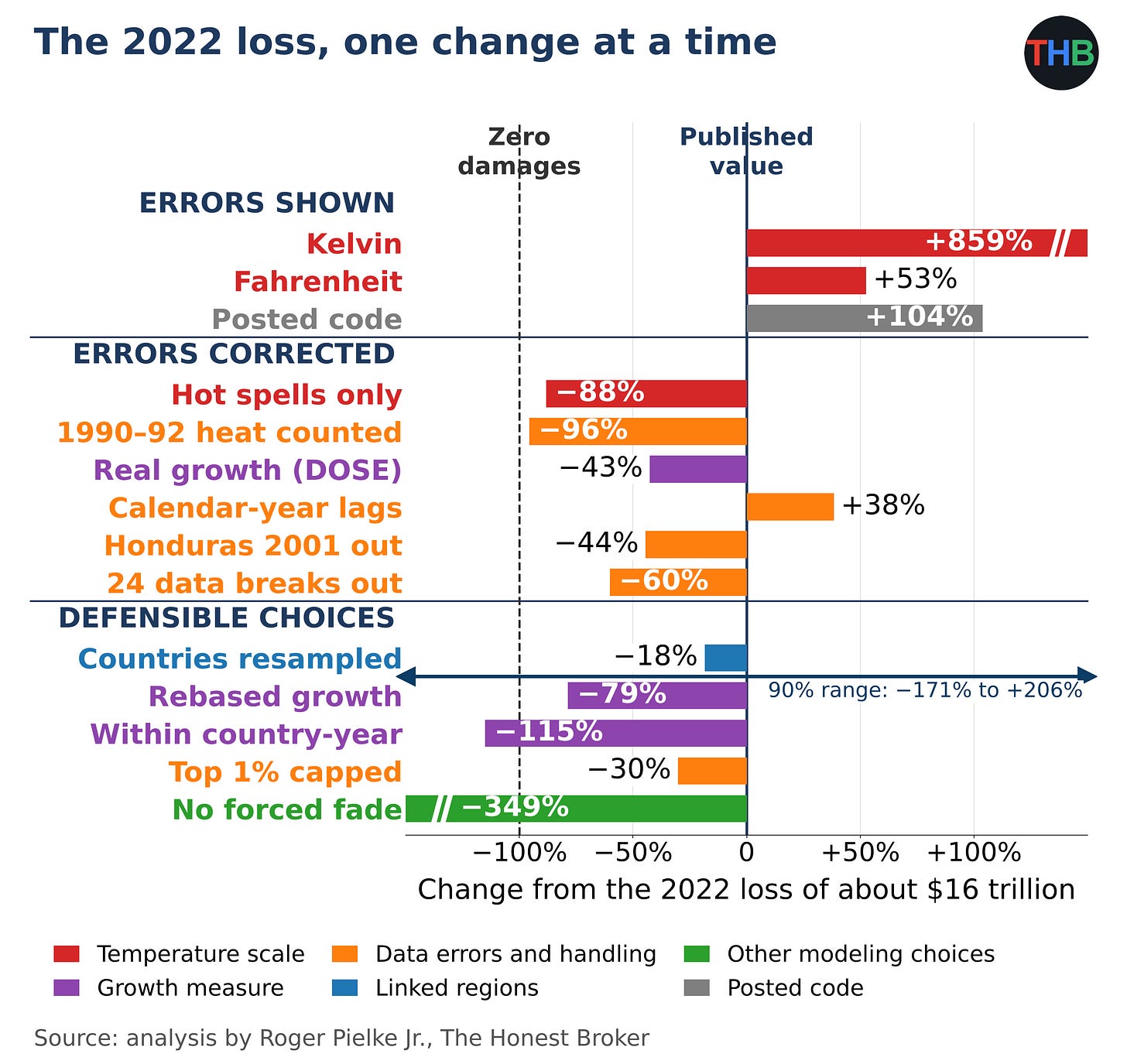
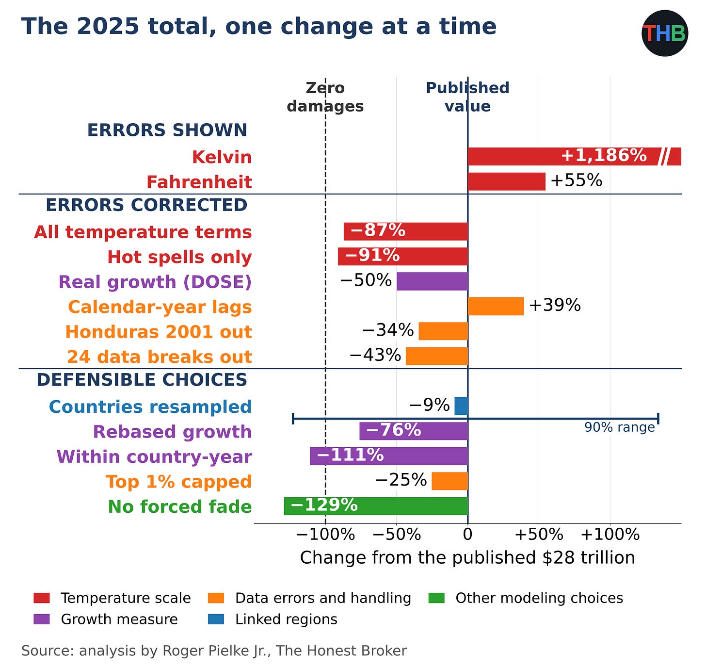
In the 2025 figure above, I start from the published $28 trillion and change one step at a time, and in each bar I show the percent change from that single change. In the top group, I show the error in the temperature scale: the same calculation in Kelvin and Fahrenheit.

In the middle group, I correct errors; in the bottom group, I substitute choices as reasonable as Callahan and Mankin’s choices. I color each bar by the type of problem and draw a dashed line at −100%, the point of zero loss. I found the largest swing among the choices in the fade. Callahan and Mankin force the economic harm from a hot spell to disappear within three years. When I used their statistical estimates for all six years, I got an average gain of $8 trillion in place of the $28 trillion loss, with a 90% range from a $107 trillion gain to a $133 trillion loss. The other bars are discussed in the accompanying methods document.

Blame for individual companies

Callahan and Mankin opened their paper by arguing that “the scientific case for climate liability is closed.” In their summary, they wrote that “drawing quantitative linkages between individual emitters and particularized harms is now feasible.” They offered Chevron as their example.

Taking Callahan and Mankin at face value, I tested how far Chevron’s attributed losses move under the corrected errors, methodological choices, and under Wyner and Brill’s model.

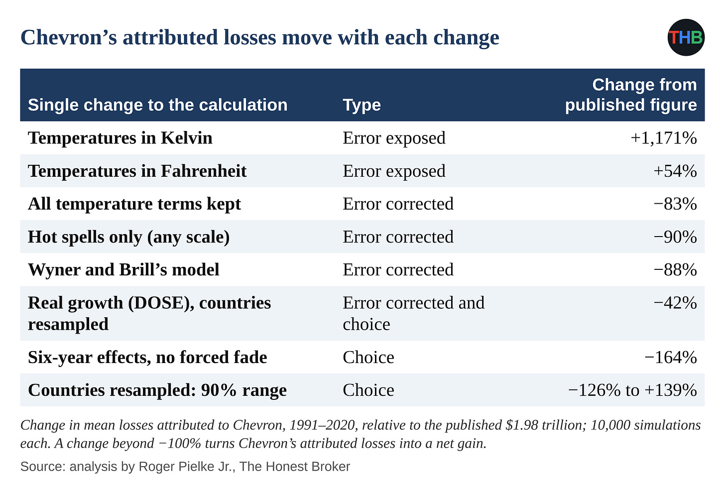
When I correct the temperature-scale error, I cut Chevron’s figure by 83% to 90%, depending on the correction. In Kelvin, I get an increase of 1,171%. Under Wyner and Brill’s model, I get a cut of 88%. Without the forced three-year fade, I get a net gain for Chevron. With country sampling alone, I get a 90% range for Chevron from −126% to +139% of the published figure.

What number would you prefer?

There are plenty to choose from and with different magnitudes and different signs.